|
|---|
![]()
Houdini Dynamics and Effects Fluid Primitives: Particles Driven from Primitive Point with FlipFluid Solver |
|---|
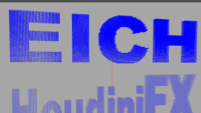
This document demonstrates a workflow that uses the position of points in geometry primitives as source and destination parameters for a flip fluid particle simulation (Figure 01: Click caption). To summarize: two seperate primitives are dropped to scene. From these primitives, points are isolated, called, and forced from primitive A to the point position's of primitive B. This is done using an attractor SOP. From this source and target simulation bgeo files are baked. These bgeos are then used as source reference in a flip fluid solver. This simple method creates from the point translation animation a fluid substance simulation. The result provides fluid simulation of primitive A morphing to the position and volume of primitive B. |
Figure 01: Fluid Primitive Simulation |
|
|---|---|---|
An important step after converting the primitive objects into points (via pointsfromvolume node) is to ensure that the primitives have an equal amount of points. |
|
|
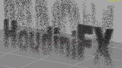
With the points for each primitive equal and sorted, a popnetwork can be dropped to continue the workflow. The popnetwork used will create a proxy simulation. |
|
|
If sorted properly, for example, point 1 in primitive A is located in the upper left of that primitive. A particle will be born from that spot and float over to the upper left corner of primitive B. This results mimicks a rough draft of a fluid sim. The Flip Fluid Solver is located in the Particle Fluids tab shelf button. This Houdini tool will take the popnetwork and create a simulation from it. The result is a dopnetwork and fluid sim node both dropped to the nodeview window. |
|
|
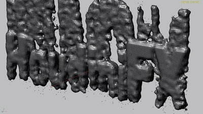
The dopnet contains the parameters of the particles, within force, birth, and death parameters can all be adjusted. The second node that was dropped is the actual fluid sim desired for render. It contains the surfacing and volume properties of the fluid solver. This network imports the dopnet and behaves accordingly (Figure 05). Note: In the sequence there is excess particles that pass primitive B to collide with a ground plane. Since this write-up explores only primitive point to point simulation it was exluded. However briefly: a random group of particles from the simulation can be copied from the dopnet and simmed in a new popnet using gravity as force. From there the process of referencing for a flip fluid is done again. |
|