|
|---|
![]()
Houdini Dynamics and Effects Magnet Force: Metaball Dynamics Simulation (with Billiard Balls) |
|---|
This workflow demonstrates the use of magent force simulation with Houdini. The result is a strong and fluid movement of objects to and from origin. For this example, spheres are pushed and pulled using a magnet force dop network. Once keyframed, the resulting animation exhibits an ideal example of magnet force behavior. To enhnace visual clarity of object movement, textures in the form of cue balls are added to the geometry. Click Figure 01's caption or this link for full resolution video. |
||
|---|---|---|
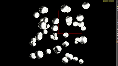
The Rigid Body Point Object shelf tool is used to scatter geometry across a number of points. |
|
|
For the source points, a scatter SOP is used to scatter points within a volume. This SOP computes nearest point ( Average of N nearest ). |
|
|
|
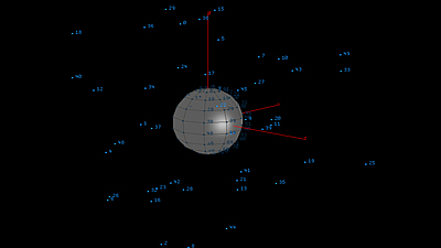
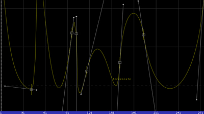
The metaball is transformed slightly. Since the ball serves as the center in which the spheres will attract, moving it even slightly will have a visible result on the final simulation. The method for translating the metaball used in this example is a Motion Effects Chop Network. This method creates a Motion Effects Chop Network from the metaball nodes translate parms. Noise is added within this CHOP network. The application of noise to translation value can be seen in the Motion View Pane ( Figure 04 ). Once the metaball is animated, the Houdini Magnet Force shelf tool can be used. The metaball serves as the force field in which the spheres will be constrained. If Magnet Force is applied properly, a new operator called magnetforce1 will be added to the dop network tree. |
|
|
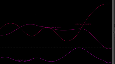
The scale of force in the magnetforce operator can be keyframed ( Figure 05 ). This parameter will adjust the proximity of the spheres to origin. This creates the push and pull aspect of the simulation. Another addition to the simulation would be another force that can slightly boost the rotation of the spheres. A uniform force operator will server for this purpose. A fraction of noise is added via the uniform force operator. This increases variation in rotation among spheres. For a final adjustment, a drag force operator is used to adjust velocity-related parameters ( for this example, Torque ). |
|
|
Patterns and textures will provide real appeal to the motion within this simulation. For this example, a custom attribute is added to each sphere with the AttribCreate operator (this is done within the instanced spheres/points geo object, after the dopimport operator). This operator applies a string parameter to each sphere. The string itself is created through concatenation of the project's working directory, an increment variable, and a filetype extension. An example of string concatenation: $HIP/img_directory. + rand($OBJID) + 1 + .png If concatentation and the file location and name conventions are consistent, a texture can will be applied randomly to each sphere from that directory. (File names, concatenation, and increment iterations must be exact. This custom attribute string that is being concatenated is the path to the image file(s). Understandable, it must be exact). Note: Another element that will really sell the motion of this simulation is motion blur. Adding velocity and object motion blur will really sell the movement of the spheres when combined with texture patterns (as this example demonstrates with cue ball textures). |
|